K-Means Clustering
Introduction
The k-Means algorithm clusters data by trying to separate samples in n groups of equal variance, minimizing a criterion known as the inertia or within-cluster sum-of-squares. This algorithm requires the number of clusters to be specified. It scales well to large number of samples and has been used across a large range of application areas in many different fields.
The k-means algorithm divides a set of N samples X into K disjoint clusters C, each described by the mean μ of the samples in the cluster. The means are commonly called the cluster “centroids”; note that they are not, in general, points from X, although they live in the same space. The k-means algorithm aims to choose centroids that minimise the inertia, or within-cluster sum of squared criterion.
The disadvantages of k-means include :
- Inertia makes the assumption that clusters are convex and isotropic, which is not always the case. It responds poorly to elongated clusters, or manifolds with irregular shapes.
- Inertia is not a normalized metric: we just know that lower values are better and zero is optimal. But in very high-dimensional spaces, Euclidean distances tend to become inflated (this is an instance of the so-called “curse of dimensionality”). Running a dimensionality reduction algorithm such as PCA prior to k-means clustering can alleviate this problem and speed up the computations.
K-means Clustering on the Enron Corpus
Enron was one of the largest US companies in 2000. At the end of 2001, it had collapsed into bankruptcy due to widespread corporate fraud, known since as the Enron scandal. A vast amount of confidential information including thousands of emails and financial data was made public after Federal investigation.
In this project, I will apply k-means clustering to the Enron financial data.
-
We first need to download the Enron Corpus (this might take a while, like more than an hour) and unzip the file (which can take a while too). There is 156 people in this dataset each one identified by their last name and the first letter of their first name.
-
Let's take a look at the data. The dataset for the project can be read as a dictionary where each key is a person and its value is a dictionnary containing all the possible feature. Here is an example of one of the entry :
{'ALLEN PHILLIP K': {'bonus': 4175000, 'deferral_payments': 2869717, 'deferred_income': -3081055, 'director_fees': 'NaN', 'email_address': 'phillip.allen@enron.com', 'exercised_stock_options': 1729541, 'expenses': 13868, 'from_messages': 2195, 'from_poi_to_this_person': 47, 'from_this_person_to_poi': 65, 'loan_advances': 'NaN', 'long_term_incentive': 304805, 'other': 152, 'poi': False, 'restricted_stock': 126027, 'restricted_stock_deferred': -126027, 'salary': 201955, 'shared_receipt_with_poi': 1407, 'to_messages': 2902, 'total_payments': 4484442, 'total_stock_value': 1729541} } -
I will first perfom k-means based on just two features, "salary" and "exercised_stock_options".
### Modified from: Udacity - Intro to Machine Learning

import pickle
from feature_format import featureFormat, targetFeatureSplit
from sklearn.model_selection import train_test_split
from sklearn.preprocessing import MinMaxScaler
import matplotlib.pyplot as plt

##########################################################################
### Split data

### A pickle document was created by the instructors of the course.
### To find it, see the full project on github
dictionary = pickle.load( open("../final_project/final_project_dataset_modified.pkl", "r") )

### Create a list of features with the first one being "poi"
poi  = "poi"
feature_1 = "salary"
feature_2 = "exercised_stock_options"
features_list = [poi, feature_1, feature_2]

### FeatureFormat converts data from the dictionary format to an
### (n x k) python list that's ready for training an sklearn algorithm
data = featureFormat(dictionary, features_list, remove_any_zeroes=True)

### targetFeatureSplit separates out the first feature (should be the target)
### from the others. The function returns targets in in its own list
### and all of the other features in a separate list
poi, finance_features = targetFeatureSplit( data )

### Feature scaling
scaler = MinMaxScaler(feature_range=(0, 1), copy=True)
scaler.fit(finance_features)
finance_features = scaler.transform(finance_features)

##########################################################################
### Draw the scatterplot

for f1, f2 in finance_features:
    plt.scatter( f1, f2 )

### Add axis labels
plt.xlabel(features_list[1])
plt.ylabel(features_list[2])
plt.savefig("test.png")
plt.show()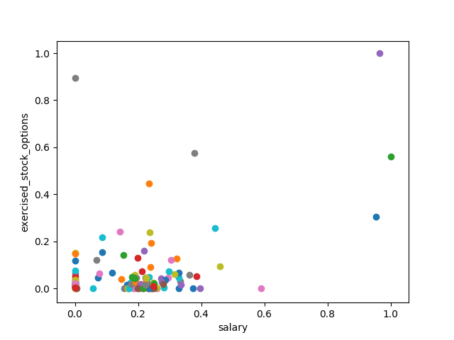
Scaled repartition of the people and their "exercised_stock_options" with respect to their "salary"
-
The class sklearn.cluster.KMeans() was used for clustering.
### Modified from: Udacity - Intro to Machine Learning

from sklearn.cluster import KMeans

kmeans = KMeans(n_clusters=2, random_state=0).fit(finance_features)

### Fitting linear model on the training set
kfit = kmeans.fit(finance_features)

### Cluster prediction
pred = kmeans.predict(finance_features)

##########################################################################
### Draw the scatterplot with n_clusters

for ii, pp in enumerate(pred):
    plt.scatter(features[ii][0], features[ii][1], color=colors[pred[ii]])

### Add axis labels
plt.xlabel(features_list[1])
plt.ylabel(features_list[2])
plt.savefig("test.png")
plt.show()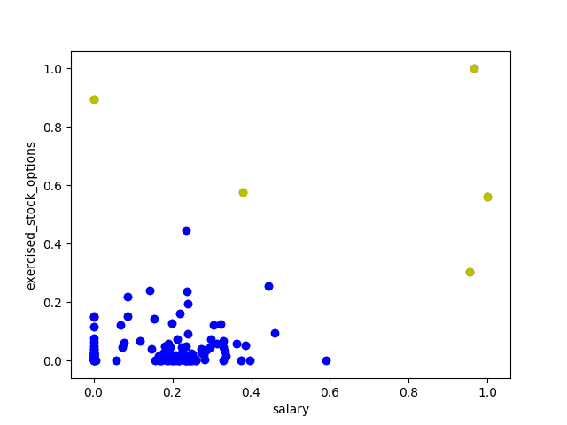
K-means cluster with 2 features
feature1 = "salary", feature2 = "exercised_stock_options"
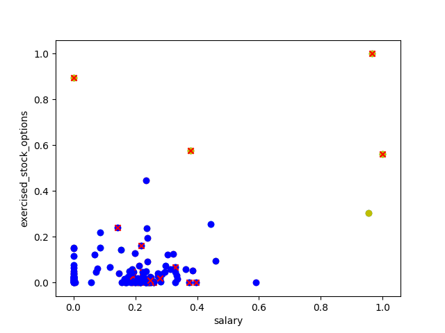
K-means cluster with 2 features with marked "poi"
Red crosses show "poi"
Two clusters are identified in blue and yellow. The scheme with marked "poi" shows that the yellow cluster identify some "poi" but still a lot of them fall into the blue cluster. More features might be necessary for better clustering.
Accuracy calculations for this clusters are :
- Global Accuracy = 87.903 %
- Poi Accuracy = 22.222 %
- Non-Poi Accuracy = 99.057 %
Global accuracy reaches 87.903 % but poi accuracy is pretty low, which means that the cluster is not effective at finding poi. On the other hand, the Non-Poi accuracy is high, 99.057 %, meaning that we are less suceptible of getting false positives. -
A third feature "total_payments" is taken into account.
### Modified from: Udacity - Intro to Machine Learning

import pickle
from feature_format import featureFormat, targetFeatureSplit
from sklearn.model_selection import train_test_split
from sklearn.preprocessing import MinMaxScaler
import matplotlib.pyplot as plt

##########################################################################
### Split data

dictionary = pickle.load( open("../final_project/final_project_dataset_modified.pkl", "r") )

poi  = "poi"
feature_1 = "salary"
feature_2 = "exercised_stock_options"
feature_3 = "total_payments"
features_list = [poi, feature_1, feature_2, feature_3]

data = featureFormat(dictionary, features_list, remove_any_zeroes=True)
poi, finance_features = targetFeatureSplit( data )

scaler = MinMaxScaler(feature_range=(0, 1), copy=True)
scaler.fit(finance_features)
finance_features = scaler.transform(finance_features)

##########################################################################
### Draw the scatterplot

fig = plt.figure()
ax = fig.add_subplot(111, projection='3d')

for f1, f2, f3 in finance_features:
    ax.scatter( f1, f2, f3 )

### Add labels
ax.set_xlabel(features_list[1])
ax.set_ylabel(features_list[2])
ax.set_zlabel(features_list[3])
plt.savefig("test.png")
plt.show()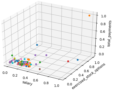
Scaled repartition of the people with 3 features
feature1 = "salary", feature2 = "exercised_stock_options", feature3 = "total_payments"
-
Clustering with three features (n_clusters = 2)
### Modified from: Udacity - Intro to Machine Learning

from sklearn.cluster import KMeans

kmeans = KMeans(n_clusters=2, random_state=0).fit(finance_features)

### Fitting linear model on the training set
kfit = kmeans.fit(finance_features)

### Cluster prediction
pred = kmeans.predict(finance_features)

##########################################################################
### Draw the scatterplot with n_clusters

fig = plt.figure()
ax = fig.add_subplot(111, projection='3d')

colors = ['b', 'y']
for ii, pp in enumerate(pred):
    plt.scatter(features[ii][0], features[ii][1], features[ii][2] color=colors[pred[ii]])

### Add axis labels
ax.set_xlabel(features_list[1])
ax.set_ylabel(features_list[2])
ax.set_zlabel(features_list[3])

plt.savefig("test.png")
plt.show()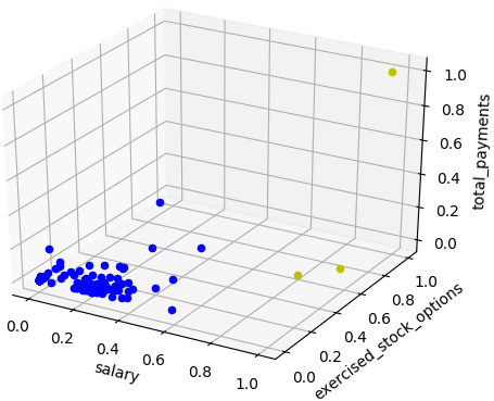
K-means cluster (n_clusters = 2) with 3 features
feature1 = "salary", feature2 = "exercised_stock_options", feature3 = "total_payments"
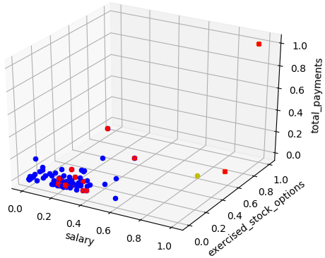
K-means cluster (n_clusters = 2) with 3 features with marked "poi"
Red crosses show "poi"
Clustering (n_clusters = 2) with the 3 features "salary", "exercised_stock_options" and "total_payments" makes some point from the yellow to switch into the blue group. Accuracy calculations are:
- Global Accuracy = 87.770 %
- Poi Accuracy = 11.111 %
A Global Accuracy of 87.770 % shows that the clustering does a decent job at finding if a person is or is not a "poi". However, when looking only at the "poi" feature the accuracy drops to 11.111 % meaning that the clustering is not very good at finding "poi". -
Clustering with three features (n_clusters = 3)
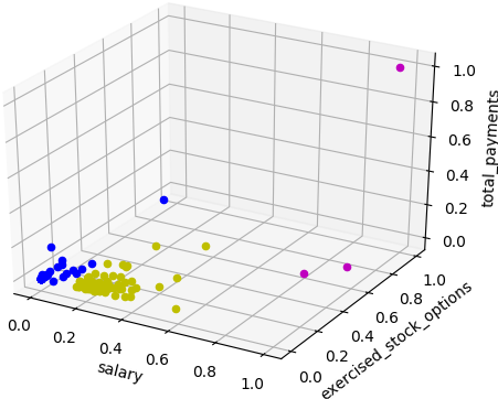
K-means cluster (n_clusters = 3) with 3 features
feature1 = "salary", feature2 = "exercised_stock_options", feature3 = "total_payments"
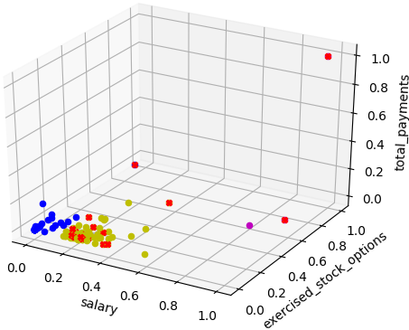
K-means cluster (n_clusters = 3) with 3 features with marked "poi"
Red crosses show "poi"
Clustering with n_clusters = 3 when the outcome expected is binary (is "poi" or is not "poi") might seem odd. However, the classification can be considered as a gradient as of probability where we consider three states :
- Blue : low probability poi
- Yellow : probable poi
- Purple : high probability poi
Accuracy calculations for this clusters are :- Global Accuracy = 50.360 %
- Poi Accuracy (when considering only probable poi) = 83.333 %
- Poi Accuracy (when considering both probable poi and high probability poi)= 94.444 %
- Non-Poi Accuracy = 43.802 %
The Global Accuracy drops drastically to 50.360 % showing that the cluster is more prone to get false positive. However, the poi Accuracy rises to 94.444 % when considering both probable poi and high probability poi. One remarkable thing about this clustering is that the low probability poi cluster predicts non poi with an accuracy of 98.148 %.