Support Vector Machine

Introduction

Support vector machines (SVMs) are a set of supervised learning methods used for classification, regression and outliers detection.

The advantages of support vector machines are :

Effective in high dimensional spaces.
Still effective in cases where number of dimensions is greater than the number of samples.
Uses a subset of training points in the decision function (called support vectors), so it is also memory efficient.
Versatile: different Kernel functions can be specified for the decision function. Common kernels are provided, but it is also possible to specify custom kernels.

The disadvantages of support vector machines include :

If the number of features is much greater than the number of samples, avoid over-fitting in choosing Kernel functions and regularization term is crucial.
SVMs do not directly provide probability estimates, these are calculated using an expensive five-fold cross-validation.

In the following projects, the class sklearn.svm.SVC() will be used. Several parameters can be set in this function such as the Kernel, gamma and C.

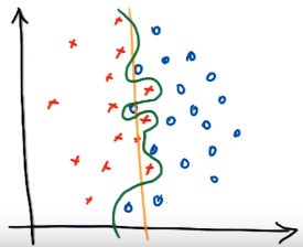
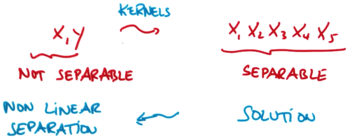
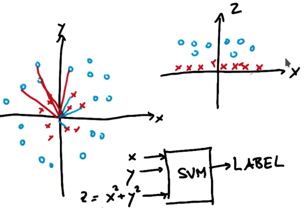
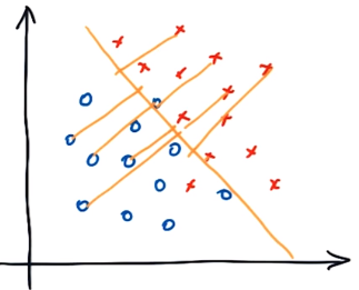
C: (Default = 1.0) Controls the tradeoff between smooth decision boundary and classifying training points correctly. A large value of C will allow to include more training points therefore leading to a more intricate boundary. Here in the scheme the orange line represents a low value of C and the green line represents a high value of C (more on Udacity).

Kernel: (default = 'rbf') Can be 'linear', 'poly', 'rbf', 'sigmoid', 'precomputed' or a callable. It's a function that takes a low dimensional input space or feature space and map it to a higher dimensional space. Therefore something that is not linearly separable can be turned into a separable problem (more on Udacity).

gamma: (Default = auto) Defines how far the influence of a single training example reaches. A High gamma value means only the closest points to the decision boundary will carry the weigth leading to a smoother boundary. One the other hand a low gamma value means even the points far away from the decision boundary have a weigth leading to a more wiggly boundary (more on Udacity).

Support vector machine for self-driving car

We want to train a car to decide weither or not it can drive faster or if it should slow down depending on the terrain. Two features will be taken into account in this project :

Bumpiness: the more bumps on the road, the slower the car should go.
Steepness: the steeper the road, the slower the car should go.

I will describe the procedure I went through step by step using Support Vector Machine (SVM) as classifiers.

We first need to create a dataset of terrain with the features bumpiness and steepness along with a label "fast" or "slow". From this labeled dataset, we will be able to build a decision tree to help the car make it's decision : "Should I go slow or fast?"

                                
### Modified from: Udacity - Intro to Machine Learning

import random
def makeTerrainData(n_points):
    random.seed(42)
    ### generate random data for both features 'grade' and 'bumpy' with an error
    grade = [random.random() for ii in range(0,n_points)]
    bumpy = [random.random() for ii in range(0,n_points)]
    error = [random.random() for ii in range(0,n_points)]

    ### data are labeled depending on their features and error.
    ### label "slow" if labels = 1.0 
    ### label "fast" if labels = 0.0
    labels = [round(grade[ii]*bumpy[ii]+0.3+0.1*error[ii]) for ii in range(0,n_points)]

    ### adjust labels for extreme cases (>0.8) of bumpiness or steepness
    for ii in range(0, len(y)):
        if grade[ii]>0.8 or bumpy[ii]>0.8:
            labels[ii] = 1.0

    ### split into train set (75% of data generated) and test sets (25% of data generated)
    features = [[gg, ss] for gg, ss in zip(grade, bumpy)]
    split = int(0.75*n_points)
    features_train = features[0:split]
    features_test  = features[split:]
    labels_train = labels[0:split]
    labels_test  = labels[split:]

    return features_train, labels_train, features_test, labels_test

The outputs are as follows for n_points = 10 :

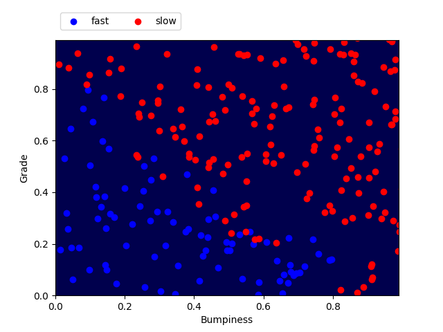
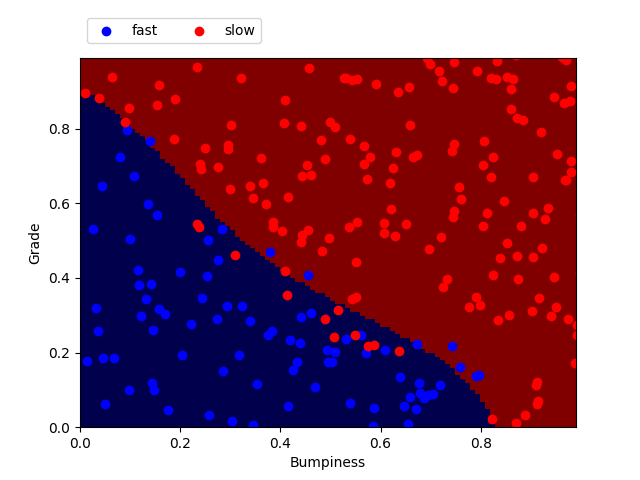
features_train		labels_train	features_test		labels_test
grade	bumpiness	slow = 1.0 \| fast = 0.0	grade	bumpiness	slow = 1.0 \| fast = 0.0
0.64	0.22	1.0	0.09	0.59	0.0
0.03	0.51	0.0	0.42	0.81	1.0
0.28	0.03	0.0	0.03	0.01	0.0
0.22	0.20	0.0
0.74	0.64	1.0
0.68	0.54	1.0
0.89	0.22	1.0

For n_points = 1000, we get the following repartition of test points. We consider the feature 'bumpiness' on the x-axis and 'grade' on the y axis. Each feature in a gradient between 0 and 1. Each point previously generated has two coordinates bumpiness and grade. When we plot the test points (features_test) - representing 25% of our generated data - we can see the pattern separating the points labeled 'slow' and 'fast'.

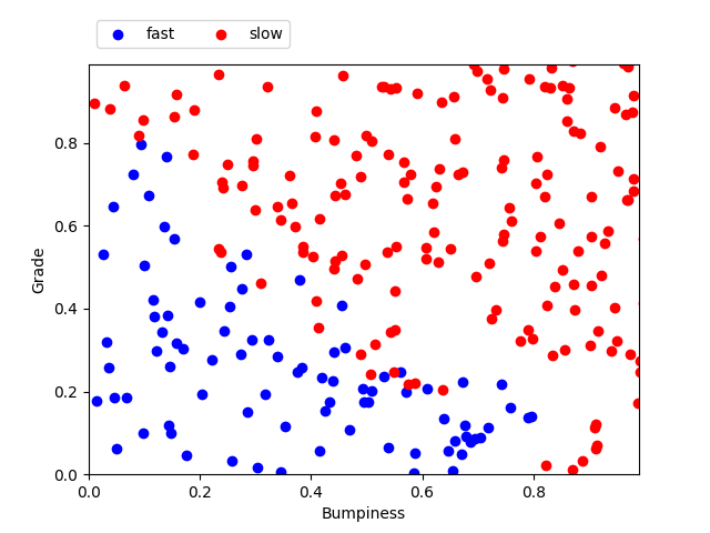
Testing set plotted with their labels

Testing set includes all features_test (grade, bumpiness) with their labels_test (slow or fast)

Now with our training set (features_train), we can train our classifier to predict a point's label depending on its features. We will use the class sklearn.svm.SVC(). It can take several parameters, but we will only focus on C, kernel and gamma.

                                
from prep_terrain_data import makeTerrainData
from sklearn.svm import SVC
from sklearn.metrics import accuracy_score

### generate the dataset for 1000 points (see previous code)
features_train, labels_train, features_test, labels_test = makeTerrainData(1000)

### create the classifier
clf = SVC(kernel='rbf', C=10000.0)

### fit the training set
clf.fit(features_train, labels_train)

### now let's make predictions on the test set
prediction = clf.predict(features_test)

### measure of the accuracy score by comparing the prediction with the actual labels of the testing set
accuracy = accuracy_score(labels_test, pred)

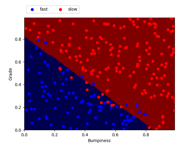
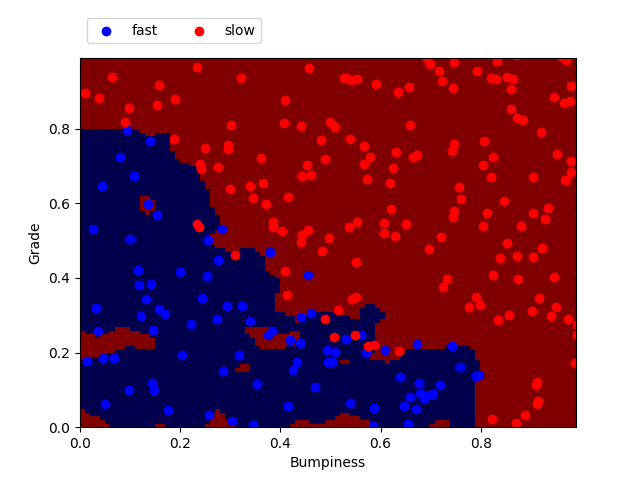
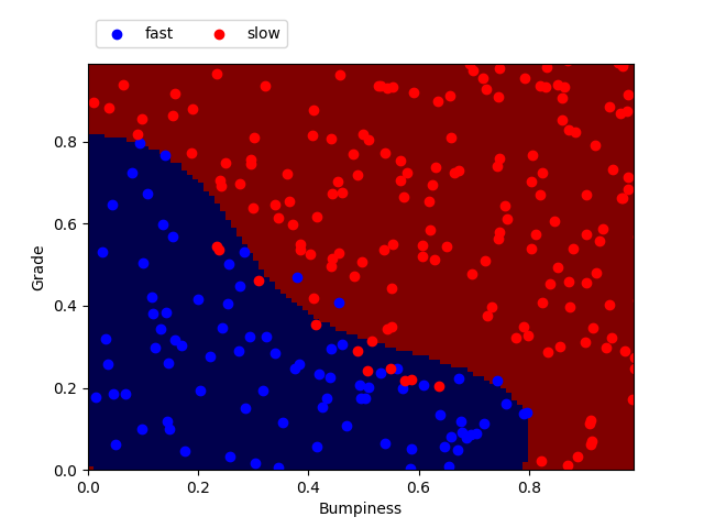
Here I plotted the points from the testing set (features_test) with their labels (labels_test). On top is the prediction made by the classifier after fitting on the training set. We can play with the previously cited features to find the best accuracy.

Kernel and gamma

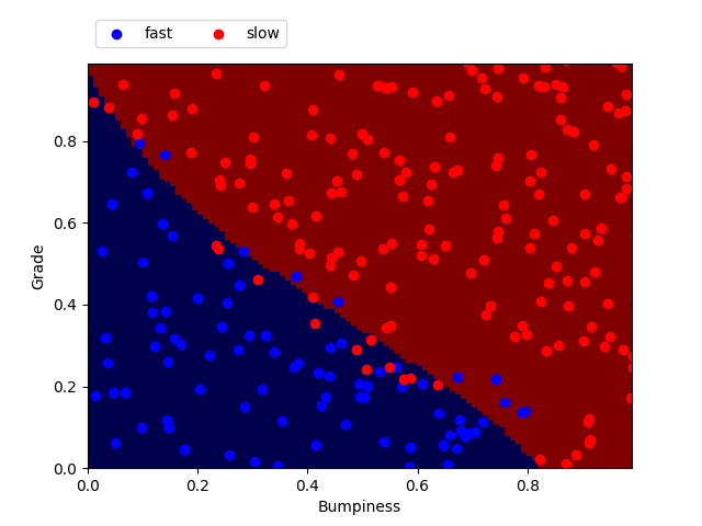
SVM with kernel = 'linear'

C = 1, gamma = 1

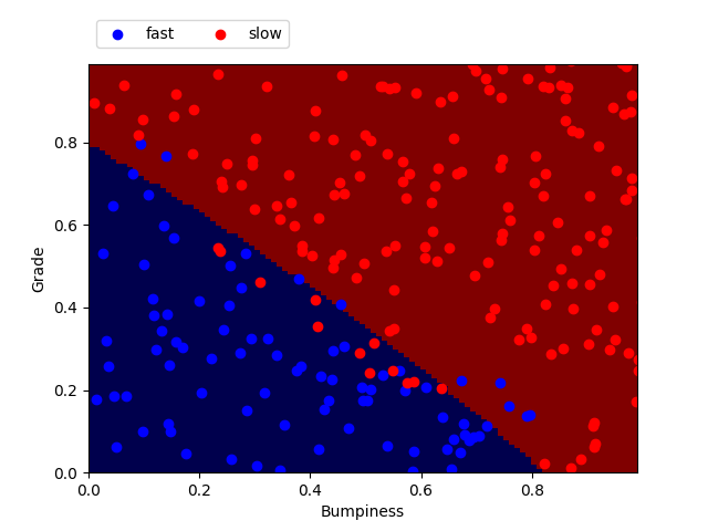
SVM with kernel = 'rbf'

C = 1, gamma = 1

SVM with kernel = 'poly'

C = 1, gamma = 1

SVM with kernel = 'sigmoid'

C = 1, gamma = 1

Kernel gamma = 1 C = 1	Training time (sec)	Predict time (sec)	Accuracy
linear	0.004	0.001	0.920
rbf	0.008	0.002	0.916
poly	0.004	0.001	0.920
sigmoid	0.012	0.003	0.900

SVM with kernel = 'linear'

C = 1, gamma = 1000

SVM with kernel = 'rbf'

C = 1, gamma = 1000

SVM with kernel = 'poly'

C = 1, gamma = 1000

SVM with kernel = 'sigmoid'

C = 1, gamma = 1000

Kernel gamma = 1000 C = 1	Training time (sec)	Predict time (sec)	Accuracy
linear	0.004	0.001	0.920
rbf	0.044	0.006	0.924
poly	61.041	0.001	0.912
sigmoid	0.008	0.002	0.664

The C parameter

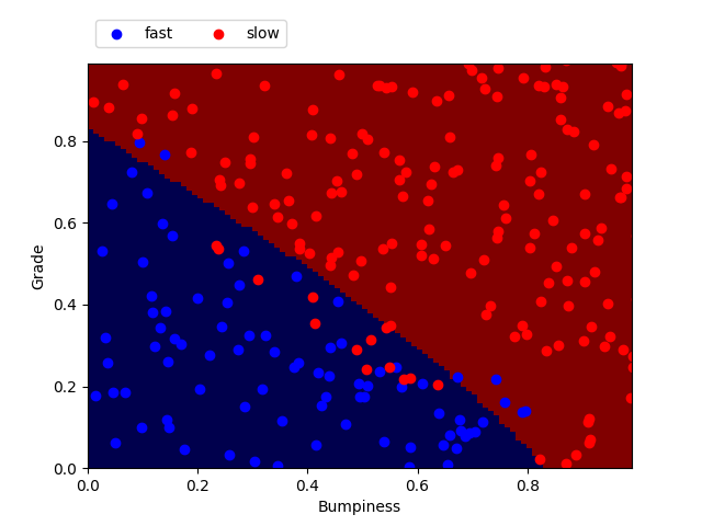
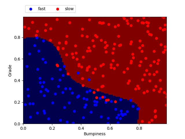
SVM with C = 1

kernel = 'rbf', gamma = default

SVM with C = 1 000

kernel = 'rbf', gamma = default

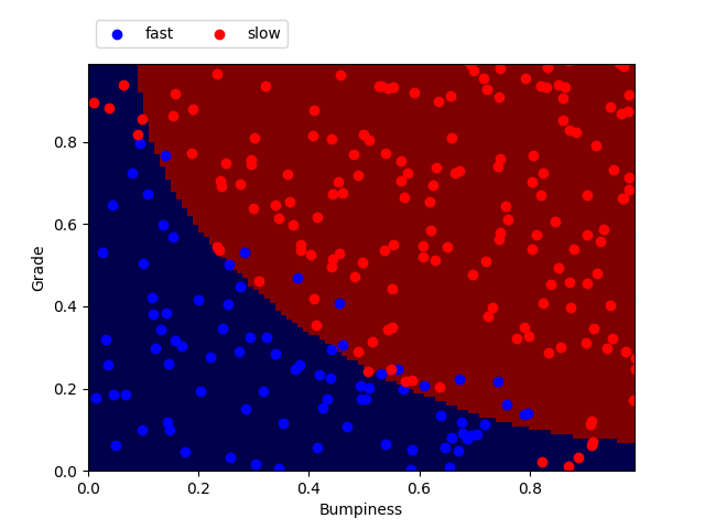
SVM with C = 10 000

kernel = 'rbf', gamma = default

SVM with C = 1 000 000

kernel = 'rbf', gamma = default

C gamma = default Kernel = 'rbf'	Training time (sec)	Predict time (sec)	Accuracy
1	0.009	0.002	0.920
100	0.010	0.001	0.916
1 000	0.012	0.001	0.924
10 000	0.021	0.001	0.932
100 000	0.132	0.001	0.944
1 000 000	1.473	0.001	0.948

Identifying emails authors with SVM

Enron was one of the largest US companies in 2000. At the end of 2001, it had collapsed into bankruptcy due to widespread corporate fraud, known since as the Enron scandal. A vast amount of confidential information including thousands of emails and financial data was made public after Federal investigation.

In this project, I will apply SVM to identify authors of emails in the Enron Corpus.

A big first part of the project is the preprocessing of emails which is described in more details here.

Once the emails are preprocessed and separated into a training and a testing set, the class sklearn.svm.SVC() can be used.

                                        
from sklearn.svm import SVC
def svm_email(features_train, features_test, labels_train, labels_test):
    clf = SVC(kernel='rbf', C=10000)
    t0 = time()
    clf.fit(features_train, labels_train)
    print ("svm training time :", round(time() - t0, 3), "s")
    t0 = time()
    pred = clf.predict(features_test)
    print ("svm predict time :", round(time() - t0, 3), "s")
    accuracy = accuracy_score(labels_test, pred)
    print ("svm accuracy :", accuracy)

def main():
    from_sara_file = "from_sara.txt"
    from_chris_file = "from_chris.txt"
    word_data, from_data = preprocess_email(from_sara_file, from_chris_file)
    features_train, features_test, labels_train, labels_test = vectorize(word_data, from_data)
    svm_email(features_train, features_test, labels_train, labels_test)
    
    if __name__ == '__main__':
        main()

Classification algorithm	Training time (sec)	Predict time (sec)	Accuracy
SVM	101.02	10.511	99.203