Decision Trees
Introduction
The advantages of decision trees include :
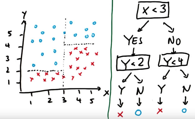
- Simple to understand and to interpret. Trees can be visualised.
- Requires little data preparation. Other techniques often require data normalisation, dummy variables need to be created and blank values to be removed.
- The cost of using the tree (i.e., predicting data) is logarithmic in the number of data points used to train the tree.
- Able to handle both numerical and categorical data. Other techniques are usually specialised in analysing datasets that have only one type of variable.
- Able to handle multi-output problems.
- Uses a white box model. If a given situation is observable in a model, the explanation for the condition is easily explained by boolean logic. By contrast, in a black box model (e.g., in an artificial neural network), results may be more difficult to interpret.
- Possible to validate a model using statistical tests. That makes it possible to account for the reliability of the model.
- Performs well even if its assumptions are somewhat violated by the true model from which the data were generated.
The disadvantages of decision trees include :
- Decision-tree learners can create over-complex trees that do not generalise the data well. This is called overfitting. Playing with parameters like minimum number of samples required at a leaf node or setting the maximum depth of the tree are necessary to avoid this problem.
- Decision trees can be unstable because small variations in the data might result in a completely different tree being generated. This problem is mitigated by using decision trees within an ensemble.
- There are concepts that are hard to learn because decision trees do not express them easily, such as XOR, parity or multiplexer problems.
- Decision tree learners create biased trees if some classes dominate. It is therefore recommended to balance the dataset prior to fitting with the decision tree.
Decision trees for self-driving car
We want to train a car to decide weither or not it can drive faster or if it should slow down depending on the terrain. Two features will be taken into account in this project :
- Bumpiness: the more bumps on the road, the slower the car should go.
- Steepness: the steeper the road, the slower the car should go.
I will describe the procedure I went through step by step using decision trees as classifiers.
-
We first need to create a dataset of terrain with the features bumpiness and steepness along with a label "fast" or "slow". From this labeled dataset, we will be able to build a decision tree to help the car make it's decision : "Should I go slow or fast?"
### Modified from: Udacity - Intro to Machine Learning

import random
def makeTerrainData(n_points):
    random.seed(42)
    ### generate random data for both features 'grade' and 'bumpy' with an error
    grade = [random.random() for ii in range(0,n_points)]
    bumpy = [random.random() for ii in range(0,n_points)]
    error = [random.random() for ii in range(0,n_points)]

    ### data are labeled depending on their features and error.
    ### label "slow" if labels = 1.0
    ### label "fast" if labels = 0.0
    labels = [round(grade[ii]*bumpy[ii]+0.3+0.1*error[ii]) for ii in range(0,n_points)]

    ### adjust labels for extreme cases (>0.8) of bumpiness or steepness
    for ii in range(0, len(y)):
        if grade[ii]>0.8 or bumpy[ii]>0.8:
            labels[ii] = 1.0

    ### split into train set (75% of data generated) and test sets (25% of data generated)
    features = [[gg, ss] for gg, ss in zip(grade, bumpy)]
    split = int(0.75*n_points)
    features_train = features[0:split]
    features_test  = features[split:]
    labels_train = labels[0:split]
    labels_test  = labels[split:]

    return features_train, labels_train, features_test, labels_test
The outputs are as follows for n_points = 10 :
features_train labels_train features_test labels_test grade bumpiness slow = 1.0 | fast = 0.0 grade bumpiness slow = 1.0 | fast = 0.0 0.64 0.22 1.0 0.09 0.59 0.0 0.03 0.51 0.0 0.42 0.81 1.0 0.28 0.03 0.0 0.03 0.01 0.0 0.22 0.20 0.0 0.74 0.64 1.0 0.68 0.54 1.0 0.89 0.22 1.0 For n_points = 1000, we get the following repartition of test points. We consider the feature 'bumpiness' on the x-axis and 'grade' on the y axis. Each feature in a gradient between 0 and 1. Each point previously generated has two coordinates bumpiness and grade. When we plot the test points (features_test) - representing 25% of our generated data - we can see the pattern separating the points labeled 'slow' and 'fast'.
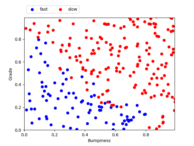
Testing set plotted with their labels
Testing set includes all features_test (grade, bumpiness) with their labels_test (slow or fast)
-
Now with our training set (features_train), we can train our classifier to predict a point's label depending on its features. We will use the class sklearn.tree.DecisionTreeClassifier(). It can take several parameters, but we will only focus on the min_samples_split which determines the number of samples ending up in each leaves of the tree.
from prep_terrain_data import makeTerrainData
from sklearn import tree
from sklearn.metrics import accuracy_score

### generate the dataset for 1000 points (see previous code)
features_train, labels_train, features_test, labels_test = makeTerrainData(1000)

### create the classifier. Here min_samples_split is set to 2.
clf = tree.DecisionTreeClassifier(min_samples_split= 2)

### fit the training set
clf.fit(features_train, labels_train)

### now let's make predictions on the test set
prediction = clf.predict(features_test)

### measure of the accuracy score by comparing the prediction with the actual labels of the testing set
accuracy = accuracy_score(labels_test, pred)
Here I plotted the points from the testing set (features_test) with their labels (labels_test). On top is the prediction made by the classifier after fitting on the training set. We can see that the classifier makes a pretty good job at separating the points.
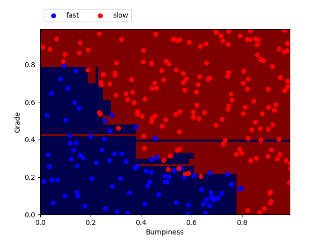
Decision tree with min_samples_split = 2
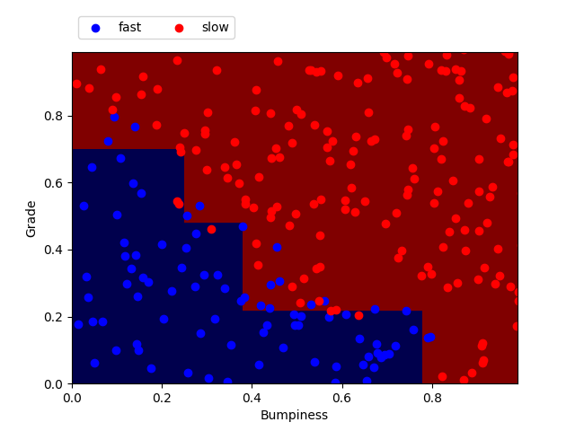
Decision tree with min_samples_split = 50
min_samples_split Training time (sec) Predict time (sec) Accuracy 2 0.001 0.000 0.908 50 0.001 0.000 0.912 Here we can see that the accuracy is higher when min_samples_split = 50 than when min_samples_split=2. A low min_samples_split means more edges to the tree so a more precise classification on the training set but not necessarily more accuracy on the test set because this can lead to overfitting. We need to be aware of the fine tuning of parameters in order to improve prediction.
Identifying emails authors with Decision trees
Enron was one of the largest US companies in 2000. At the end of 2001, it had collapsed into bankruptcy due to widespread corporate fraud, known since as the Enron scandal. A vast amount of confidential information including thousands of emails and financial data was made public after Federal investigation.
In this project, I will apply decision trees to identify authors of emails in the Enron Corpus.
-
A big first part of the project is the preprocessing of emails which is described in more details here.
-
Once the emails are preprocessed and separated into a training and a testing set, the class sklearn.tree.DecisionTreeClassifier() can be used.
from sklearn import tree
def dt_email (features_train, features_test, labels_train, labels_test):

    clf = tree.DecisionTreeClassifier(min_samples_split=40)
    t0 = time()
    clf.fit(features_train, labels_train)
    print ("decision tree training time :", round(time() - t0, 3), "s")

    t0 = time()
    pred = clf.predict(features_test)
    print ("decision tree predict time :", round(time() - t0, 3), "s")

    accuracy = accuracy_score(labels_test, pred)
    print ("decision tree accuracy :", accuracy)

def main():
    from_sara_file = "from_sara.txt"
    from_chris_file = "from_chris.txt"
    word_data, from_data = preprocess_email(from_sara_file, from_chris_file)
    features_train, features_test, labels_train, labels_test = vectorize(word_data, from_data)
    dt_email(features_train, features_test, labels_train, labels_test)

if __name__ == '__main__':
    main()
Classification algorithm Training time (sec) Predict time (sec) Accuracy Decision tree 61.709 0.064 98.805