Principal Component Analysis
Introduction
Principal Component Analysis (PCA) is used to decompose a multivariate dataset in a set of successive orthogonal components that explain a maximum amount of the variance.
When to use PCA ?
- Latent features : There are many features in the dataset but the hypothesis is that just some of them are actually driving the pattern
- Dimensionality reduction : Looking to make a composite feature that more directly probes the underlying phenomenon for dimensionality reduction and therefore being able to visualize high-dimensional data, reduce noise and being able to use other algorithms (regression, classification)
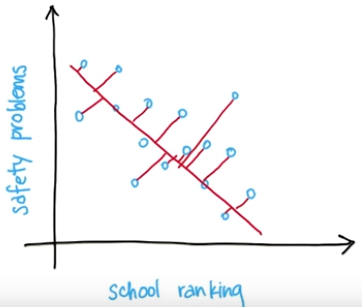
An example of dimensionality reduction can be the price of a house according to 4 features:
- Square footage
- Number of rooms
- School ranking
- Safety problems
Face Recognition with PCA (eigenfaces)
What makes facial recognition in pictures good for PCA ?
- Each pixels is a feature, meaning that pictures generally have high input dimensionality.
- Faces have patterns that could be captured in smaller number of dimensions (eyes, nose, mouth, chin...)
In this project, I will apply PCA face recognition of presidents.
-
Getting the data and generate training and testing set :
""" =================================================== Faces recognition example using eigenfaces and SVMs =================================================== The dataset used in this example is a preprocessed excerpt of the "Labeled Faces in the Wild", aka LFW_: http://vis-www.cs.umass.edu/lfw/lfw-funneled.tgz (233MB) .. _LFW: http://vis-www.cs.umass.edu/lfw/ original source: http://scikit-learn.org/stable/auto_examples/applications/face_recognition.html """ import numpy as np from sklearn.datasets import fetch_lfw_people from sklearn.model_selection import train_test_split # Download the data, if not already on disk and load it as numpy arrays lfw_people = fetch_lfw_people(min_faces_per_person=70, resize=0.4) # introspect the images arrays to find the shapes (for plotting) n_samples, h, w = lfw_people.images.shape np.random.seed(42) # for machine learning we use the data directly (as relative pixel # position info is ignored by this model) X = lfw_people.data n_features = X.shape[1] # the label to predict is the id of the person y = lfw_people.target target_names = lfw_people.target_names n_classes = target_names.shape[0] print "Total dataset size:" print "n_samples: %d" % n_samples print "n_features: %d" % n_features print "n_classes: %d" % n_classes ############################################################################### # Split into a training and testing set X_train, X_test, y_train, y_test = train_test_split(X, y, test_size=0.25, random_state=42) -
Compute the eigenfaces
from time import time
from sklearn.decomposition import PCA

# Compute a PCA (eigenfaces) on the face dataset (treated as unlabeled
# dataset): unsupervised feature extraction / dimensionality reduction
n_components = 150

print "Extracting the top %d eigenfaces from %d faces" % (n_components, X_train.shape[0])
t0 = time()
pca = PCA(n_components=n_components, whiten=True, svd_solver='randomized').fit(X_train)
print "done in %0.3fs" % (time() - t0)

eigenfaces = pca.components_.reshape((n_components, h, w))

print "Projecting the input data on the eigenfaces orthonormal basis"
t0 = time()
X_train_pca = pca.transform(X_train)
X_test_pca = pca.transform(X_test)
print "done in %0.3fs" % (time() - t0)

print ("variance ratio: ", pca.explained_variance_ratio_)
PCA orders the principal components so that the first PC gives the direction of the maximal variance, the second PC has the second largest and so on... An ordered array of all variance can be called with the attribute explained_variance_ratio_ .
Here the first three PC are :- 0.19077216
- 0.15184273
- 0.07375473
-
Train a classification model
from sklearn.svm import SVC from sklearn.model_selection import GridSearchCV # Train a SVM classification model print "Fitting the classifier to the training set" t0 = time() param_grid = { 'C': [1e3, 5e3, 1e4, 5e4, 1e5], 'gamma': [0.0001, 0.0005, 0.001, 0.005, 0.01, 0.1], } clf = GridSearchCV(SVC(kernel='rbf', class_weight='balanced'), param_grid) clf = clf.fit(X_train_pca, y_train) print "done in %0.3fs" % (time() - t0) print "Best estimator found by grid search:" print clf.best_estimator_ -
Evalutation of the model quality :
from sklearn.metrics import classification_report from sklearn.metrics import confusion_matrix print "Predicting the people names on the testing set" t0 = time() y_pred = clf.predict(X_test_pca) print "done in %0.3fs" % (time() - t0) print classification_report(y_test, y_pred, target_names=target_names) print confusion_matrix(y_test, y_pred, labels=range(n_classes)) >>> classification_report should print : precision recall f1-score support Ariel Sharon 1.00 0.62 0.76 13 Colin Powell 0.83 0.92 0.87 60 Donald Rumsfeld 0.91 0.74 0.82 27 George W Bush 0.83 0.97 0.90 146 Gerhard Schroeder 0.85 0.68 0.76 25 Hugo Chavez 1.00 0.60 0.75 15 Tony Blair 1.00 0.72 0.84 36 avg / total 0.87 0.86 0.86 322 >>> confusion_matrix should print : [[ 8 2 1 2 0 0 0] [ 0 55 0 5 0 0 0] [ 0 1 20 6 0 0 0] [ 0 4 0 142 0 0 0] [ 0 1 1 6 17 0 0] [ 0 1 0 3 2 9 0] [ 0 2 0 7 1 0 26]] ''' The confusion matrix shows for each entry names the predicted (column) and the real (line) outcome ''' -
Evalutation of the prediction :
import pylab as pl

def plot_gallery(images, titles, h, w, n_row=3, n_col=4):
    """Helper function to plot a gallery of portraits"""
    pl.figure(figsize=(1.8 * n_col, 2.4 * n_row))
    pl.subplots_adjust(bottom=0, left=.01, right=.99, top=.90, hspace=.35)
    for i in range(n_row * n_col):
        pl.subplot(n_row, n_col, i + 1)
        pl.imshow(images[i].reshape((h, w)), cmap=pl.cm.gray)
        pl.title(titles[i], size=12)
        pl.xticks(())
        pl.yticks(())

# plot the result of the prediction on a portion of the test set
def title(y_pred, y_test, target_names, i):
    pred_name = target_names[y_pred[i]].rsplit(' ', 1)[-1]
    true_name = target_names[y_test[i]].rsplit(' ', 1)[-1]
    return 'predicted: %s\ntrue:      %s' % (pred_name, true_name)

prediction_titles = [title(y_pred, y_test, target_names, i)
                         for i in range(y_pred.shape[0])]
plot_gallery(X_test, prediction_titles, h, w)

# plot the gallery of the most significative eigenfaces

eigenface_titles = ["eigenface %d" % i for i in range(eigenfaces.shape[0])]
plot_gallery(eigenfaces, eigenface_titles, h, w)

pl.show()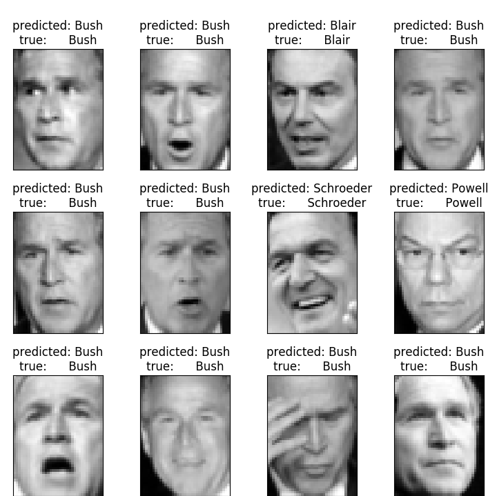
Gallery of a portion of the test set
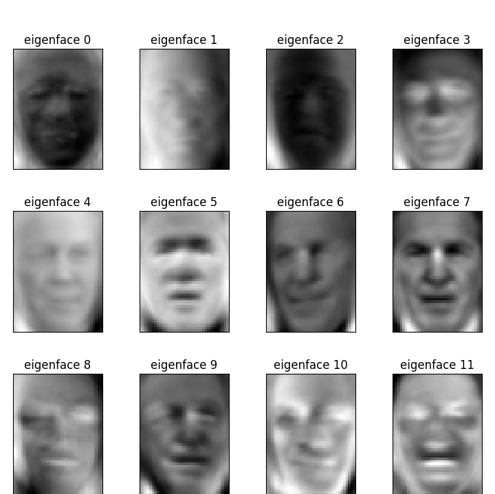
Gallery of the most significative eigenfaces
Dimension reductionality with PCA in the Enron Corpus
Enron was one of the largest US companies in 2000. At the end of 2001, it had collapsed into bankruptcy due to widespread corporate fraud, known since as the Enron scandal. A vast amount of confidential information including thousands of emails and financial data was made public after Federal investigation.
In this project, I will apply PCA to the Enron financial data.
-
We first need to download the Enron Corpus (this might take a while, like more than an hour) and unzip the file (which can take a while too). There is 156 people in this dataset each one identified by their last name and the first letter of their first name.
-
Let's take a look at the data. The dataset for the project can be read as a dictionary where each key is a person and its value is a dictionnary containing all the possible feature. Here is an example of one of the entry :
{'ALLEN PHILLIP K': {'bonus': 4175000, 'deferral_payments': 2869717, 'deferred_income': -3081055, 'director_fees': 'NaN', 'email_address': 'phillip.allen@enron.com', 'exercised_stock_options': 1729541, 'expenses': 13868, 'from_messages': 2195, 'from_poi_to_this_person': 47, 'from_this_person_to_poi': 65, 'loan_advances': 'NaN', 'long_term_incentive': 304805, 'other': 152, 'poi': False, 'restricted_stock': 126027, 'restricted_stock_deferred': -126027, 'salary': 201955, 'shared_receipt_with_poi': 1407, 'to_messages': 2902, 'total_payments': 4484442, 'total_stock_value': 1729541} } -
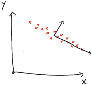
PCA calculation on two chosen features ("long_term_incentive" and "bonus")
### Modified from: Udacity - Intro to Machine Learning

import matplotlib.pyplot as plt
from sklearn.decomposition import PCA

def doPCA(data):
    pca = PCA(n_components=2)
    pca.fit(data)
    return pca

pca = doPCA(data)
print (pca.explained_variance_ratio_)
>>> Should print : [ 0.79258816  0.20741184]

first_pc = pca.components_[0]
>>> Should print : [ 0.33434446  0.94245094]

second_pc = pca.components_[1]
>>> Should print : [ 0.94245094 -0.33434446]

transformed_data = pca.transform(data)

for ii, jj in zip(transformed_data, data):
plt.scatter(first_pc[0]*ii[0], first_pc[1]*ii[0], color='r')
plt.scatter(second_pc[0]*ii[1], second_pc[1]*ii[1], color='c')
plt.scatter(jj[0], jj[1], color='m', marker="X")

plt.xlim(-0.4, 1.1)
plt.ylim(-0.4, 1.1)
plt.gca().set_aspect('equal', adjustable='box')
plt.xlabel("bonus")
plt.ylabel("long-term incentive")
plt.show()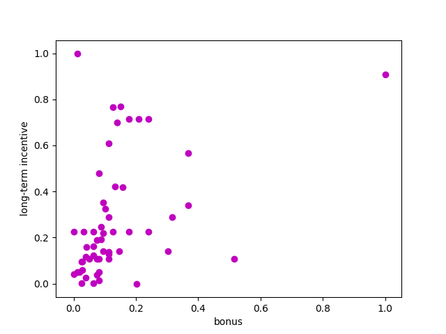
Scaled repartition of the people
feature1 = "bonus", feature2="long_term_incentive"
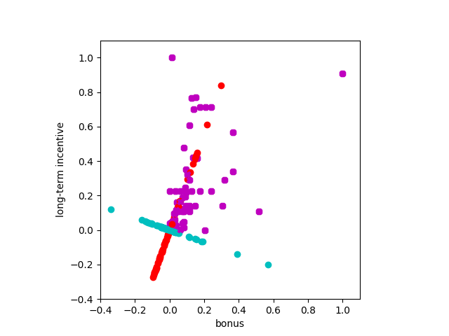
Rescaled projection of points onto first and second PC
PC1 = red, PC2 = cyan, initial dataset = magenta
The PC1 = [0.33434446, 0.94245094] and PC2 = [0.94245094, -0.33434446] are lists that contain as many principal component as specified in the parameter n_components (here n_components = 2). They are packaged into a vector that indicates the direction of x' in the xy original feature space. As PCA1 and PC2 are orthogonal, their coordinates are inversed.