Artificial Intelligence Nanodegree
Convolutional Neural Networks
Project: Write an Algorithm for a Dog Identification App
In this notebook, some template code has already been provided for you, and you will need to implement additional functionality to successfully complete this project. You will not need to modify the included code beyond what is requested. Sections that begin with '(IMPLEMENTATION)' in the header indicate that the following block of code will require additional functionality which you must provide. Instructions will be provided for each section, and the specifics of the implementation are marked in the code block with a 'TODO' statement. Please be sure to read the instructions carefully!
Note: Once you have completed all of the code implementations, you need to finalize your work by exporting the iPython Notebook as an HTML document. Before exporting the notebook to html, all of the code cells need to have been run so that reviewers can see the final implementation and output. You can then export the notebook by using the menu above and navigating to \n", "File -> Download as -> HTML (.html). Include the finished document along with this notebook as your submission.
In addition to implementing code, there will be questions that you must answer which relate to the project and your implementation. Each section where you will answer a question is preceded by a 'Question X' header. Carefully read each question and provide thorough answers in the following text boxes that begin with 'Answer:'. Your project submission will be evaluated based on your answers to each of the questions and the implementation you provide.
Note: Code and Markdown cells can be executed using the Shift + Enter keyboard shortcut. Markdown cells can be edited by double-clicking the cell to enter edit mode.
The rubric contains optional "Stand Out Suggestions" for enhancing the project beyond the minimum requirements. If you decide to pursue the "Stand Out Suggestions", you should include the code in this IPython notebook.
Why We're Here
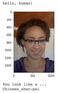
In this notebook, you will make the first steps towards developing an algorithm that could be used as part of a mobile or web app. At the end of this project, your code will accept any user-supplied image as input. If a dog is detected in the image, it will provide an estimate of the dog's breed. If a human is detected, it will provide an estimate of the dog breed that is most resembling. The image below displays potential sample output of your finished project (... but we expect that each student's algorithm will behave differently!).
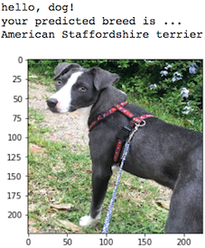
In this real-world setting, you will need to piece together a series of models to perform different tasks; for instance, the algorithm that detects humans in an image will be different from the CNN that infers dog breed. There are many points of possible failure, and no perfect algorithm exists. Your imperfect solution will nonetheless create a fun user experience!
The Road Ahead
We break the notebook into separate steps. Feel free to use the links below to navigate the notebook.
- Step 0: Import Datasets
- Step 1: Detect Humans
- Step 2: Detect Dogs
- Step 3: Create a CNN to Classify Dog Breeds (from Scratch)
- Step 4: Use a CNN to Classify Dog Breeds (using Transfer Learning)
- Step 5: Create a CNN to Classify Dog Breeds (using Transfer Learning)
- Step 6: Write your Algorithm
- Step 7: Test Your Algorithm
Step 0: Import Datasets
Import Dog Dataset
In the code cell below, we import a dataset of dog images. We populate a few variables through the use of the load_files function from the scikit-learn library:
train_files,valid_files,test_files- numpy arrays containing file paths to imagestrain_targets,valid_targets,test_targets- numpy arrays containing onehot-encoded classification labelsdog_names- list of string-valued dog breed names for translating labels
import numpy as np
import random
import cv2
import matplotlib.pyplot as plt
import sys
import os
import dlib
from skimage import io
from tqdm import tqdm
from glob import glob
from sklearn.datasets import load_files
from extract_bottleneck_features import *
from keras.callbacks import ModelCheckpoint
from keras.preprocessing import image
from keras.applications.resnet50 import ResNet50, preprocess_input, decode_predictions
from keras.utils import np_utils
from IPython.core.display import Image, display
# define function to load train, test, and validation datasets
def load_dataset(path):
data = load_files(path)
dog_files = np.array(data['filenames'])
dog_targets = np_utils.to_categorical(np.array(data['target']), 133)
return dog_files, dog_targets
# load train, test, and validation datasets
train_files, train_targets = load_dataset('dogImages/train')
valid_files, valid_targets = load_dataset('dogImages/valid')
test_files, test_targets = load_dataset('dogImages/test')
# load list of dog names
dog_names = [item[20:-1] for item in sorted(glob("dogImages/train/*/"))]
# print statistics about the dataset
print('There are %d total dog categories.' % len(dog_names))
print('There are %s total dog images.\n' % len(np.hstack([train_files, valid_files, test_files])))
print('There are %d training dog images.' % len(train_files))
print('There are %d validation dog images.' % len(valid_files))
print('There are %d test dog images.'% len(test_files))
Import Human Dataset
In the code cell below, we import a dataset of human images, where the file paths are stored in the numpy array human_files.
%matplotlib inline
# extract pre-trained face detector
face_cascade = cv2.CascadeClassifier('haarcascades/haarcascade_frontalface_alt.xml')
def boxe_face(image):
# load color (BGR) image
img = cv2.imread(image)
# convert BGR image to grayscale
gray = cv2.cvtColor(img, cv2.COLOR_BGR2GRAY)
# find faces in image
faces = face_cascade.detectMultiScale(gray)
# print number of faces detected in the image
print (faces)
print('Number of faces detected:', len(faces))
# get bounding box for each detected face
for (x,y,w,h) in faces:
# add bounding box to color image
cv2.rectangle(img,(x,y),(x+w,y+h),(0,255,0),2)
# convert BGR image to RGB for plotting
cv_rgb = cv2.cvtColor(img, cv2.COLOR_BGR2RGB)
# display the image, along with bounding box
plt.imshow(cv_rgb)
plt.show()
boxe_face(human_files[3])

random.seed(8675309)
# load filenames in shuffled human dataset
human_files = np.array(glob("lfw/*/*"))
random.shuffle(human_files)
# print statistics about the dataset
print('There are %d total human images.' % len(human_files))
Step 1: Detect Humans
We use OpenCV's implementation of Haar feature-based cascade classifiers to detect human faces in images. OpenCV provides many pre-trained face detectors, stored as XML files on github. We have downloaded one of these detectors and stored it in the haarcascades directory.
In the next code cell, we demonstrate how to use this detector to find human faces in a sample image.
Before using any of the face detectors, it is standard procedure to convert the images to grayscale. The detectMultiScale function executes the classifier stored in face_cascade and takes the grayscale image as a parameter.
In the above code, faces is a numpy array of detected faces, where each row corresponds to a detected face. Each detected face is a 1D array with four entries that specifies the bounding box of the detected face. The first two entries in the array (extracted in the above code as x and y) specify the horizontal and vertical positions of the top left corner of the bounding box. The last two entries in the array (extracted here as w and h) specify the width and height of the box.
Write a Human Face Detector
We can use this procedure to write a function that returns True if a human face is detected in an image and False otherwise. This function, aptly named face_detector, takes a string-valued file path to an image as input and appears in the code block below.
# returns "True" if face is detected in image stored at img_path
def face_detector_opencv(img_path):
img = cv2.imread(img_path)
gray = cv2.cvtColor(img, cv2.COLOR_BGR2GRAY)
faces = face_cascade.detectMultiScale(gray)
return len(faces) > 0
(IMPLEMENTATION) Assess the Human Face Detector
Question 1: Use the code cell below to test the performance of the face_detector function.
- What percentage of the first 100 images in
human_fileshave a detected human face? - What percentage of the first 100 images in
dog_fileshave a detected human face?
Ideally, we would like 100% of human images with a detected face and 0% of dog images with a detected face. You will see that our algorithm falls short of this goal, but still gives acceptable performance. We extract the file paths for the first 100 images from each of the datasets and store them in the numpy arrays human_files_short and dog_files_short.
Answer: The OpenCV's implementation of Haar feature-based cascade classifiers detects 100.0% of faces in the first 100 images in human_files and 11.0% of faces in the first 100 images in dog_files. When investigating each image where a face has been detected, we can see that for one image there is actually a human in the picture so the classifier is not making a mistake here. For 4 images, the classifier misclassifies the face of a human with a dog. For the rest of them, the classifier seems to detect faces in fur, wrinkle of fabrics...
human_files_short = human_files[:100]
dog_files_short = train_files[:100]
# Do NOT modify the code above this line.
## TODO: Test the performance of the face_detector algorithm
## on the images in human_files_short and dog_files_short.
def performance_face_detector_opencv(human_files_short, dog_files_short):
face_human = [int(face_detector_opencv(human_img)) for human_img in human_files_short]
ratio_human = sum(face_human)/len(face_human)*100
print ('{}% of faces detected in the first 100 images in human_files by OpenCV'.format(ratio_human))
face_dog = 0
for dog_img in dog_files_short:
if face_detector_opencv(dog_img):
img = cv2.imread(dog_img)
boxe_face(dog_img)
face_dog += 1
ratio_dog = face_dog/len(dog_files_short)*100
print ('{}% of faces detected in the first 100 images in dog_files by OpenCV'.format(ratio_dog))
performance_face_detector_opencv(human_files_short, dog_files_short)


Question 2: This algorithmic choice necessitates that we communicate to the user that we accept human images only when they provide a clear view of a face (otherwise, we risk having unneccessarily frustrated users!). In your opinion, is this a reasonable expectation to pose on the user? If not, can you think of a way to detect humans in images that does not necessitate an image with a clearly presented face?
Answer: When making a mobile/web application, it generally only takes a few minutes to the users to decide if they want to keep using the app or not. While mentioning beforehand that it's better to provide a clear view of a face is a good start, it would not be enough. To avoid loosing users on the first few minutes, the application should be able to satisfy the broadest audience possible. One thing we could do is to train a CNN with an augmented data set of many more human faces.
We suggest the face detector from OpenCV as a potential way to detect human images in your algorithm, but you are free to explore other approaches, especially approaches that make use of deep learning :). Please use the code cell below to design and test your own face detection algorithm. If you decide to pursue this optional task, report performance on each of the datasets.
## (Optional) TODO: Report the performance of another
## face detection algorithm on the LFW dataset
### Feel free to use as many code cells as needed.
def face_detector_dlib(image):
detector = dlib.get_frontal_face_detector()
img = cv2.imread(image)
faces = detector(img, 1)
return len(faces) > 0
def boxe_dlib(image):
detector = dlib.get_frontal_face_detector()
predictor = dlib.shape_predictor("dlib_predictor/shape_predictor_68_face_landmarks.dat")
win = dlib.image_window()
img = io.imread(image)
win.clear_overlay()
win.set_image(img)
# Ask the detector to find the bounding boxes of each face. The 1 in the
# second argument indicates that we should upsample the image 1 time. This
# will make everything bigger and allow us to detect more faces.
dets = detector(img, 1)
print("Number of faces detected: {}".format(len(dets)))
for k, d in enumerate(dets):
print("Detection {}: Left: {} Top: {} Right: {} Bottom: {}".format(
k, d.left(), d.top(), d.right(), d.bottom()))
# Get the landmarks/parts for the face in box d.
shape = predictor(img, d)
print("Part 0: {}, Part 1: {} ...".format(shape.part(0),
shape.part(1)))
# Draw the face landmarks on the screen.
win.add_overlay(shape)
win.add_overlay(dets)
def performance_face_detector_dlib(human_files_short, dog_files_short):
face_human = [int(face_detector_dlib(human_img)) for human_img in human_files_short]
ratio_human = sum(face_human)/len(face_human)*100
print ('{}% of faces detected in the first 100 images in human_files by dlib'.format(ratio_human))
face_dog = 0
for dog_img in dog_files_short:
if face_detector_dlib(dog_img):
boxe_dlib(dog_img)
face_dog += 1
ratio_dog = face_dog/len(dog_files_short)*100
print ('{}% of faces detected in the first 100 images in dog_files by dlib'.format(ratio_dog))
performance_face_detector_dlib(human_files_short, dog_files_short)
The dlib classifier detects 100.0% of faces in the first 100 images in human_files and 11.0% of faces in the first 100 images in dog_files.
Step 2: Detect Dogs
In this section, we use a pre-trained ResNet-50 model to detect dogs in images. Our first line of code downloads the ResNet-50 model, along with weights that have been trained on ImageNet, a very large, very popular dataset used for image classification and other vision tasks. ImageNet contains over 10 million URLs, each linking to an image containing an object from one of 1000 categories. Given an image, this pre-trained ResNet-50 model returns a prediction (derived from the available categories in ImageNet) for the object that is contained in the image.
# define ResNet50 model
ResNet50_model = ResNet50(weights='imagenet')
Pre-process the Data
When using TensorFlow as backend, Keras CNNs require a 4D array (which we'll also refer to as a 4D tensor) as input, with shape
$$ (\text{nb_samples}, \text{rows}, \text{columns}, \text{channels}), $$
where nb_samples corresponds to the total number of images (or samples), and rows, columns, and channels correspond to the number of rows, columns, and channels for each image, respectively.
The path_to_tensor function below takes a string-valued file path to a color image as input and returns a 4D tensor suitable for supplying to a Keras CNN. The function first loads the image and resizes it to a square image that is $224 \times 224$ pixels. Next, the image is converted to an array, which is then resized to a 4D tensor. In this case, since we are working with color images, each image has three channels. Likewise, since we are processing a single image (or sample), the returned tensor will always have shape
$$ (1, 224, 224, 3). $$
The paths_to_tensor function takes a numpy array of string-valued image paths as input and returns a 4D tensor with shape
$$ (\text{nb_samples}, 224, 224, 3). $$
Here, nb_samples is the number of samples, or number of images, in the supplied array of image paths. It is best to think of nb_samples as the number of 3D tensors (where each 3D tensor corresponds to a different image) in your dataset!
def path_to_tensor(img_path):
# loads RGB image as PIL.Image.Image type
img = image.load_img(img_path, target_size=(224, 224))
# convert PIL.Image.Image type to 3D tensor with shape (224, 224, 3)
x = image.img_to_array(img)
# convert 3D tensor to 4D tensor with shape (1, 224, 224, 3) and return 4D tensor
return np.expand_dims(x, axis=0)
def paths_to_tensor(img_paths):
list_of_tensors = [path_to_tensor(img_path) for img_path in tqdm(img_paths)]
return np.vstack(list_of_tensors)
Making Predictions with ResNet-50
Getting the 4D tensor ready for ResNet-50, and for any other pre-trained model in Keras, requires some additional processing. First, the RGB image is converted to BGR by reordering the channels. All pre-trained models have the additional normalization step that the mean pixel (expressed in RGB as $[103.939, 116.779, 123.68]$ and calculated from all pixels in all images in ImageNet) must be subtracted from every pixel in each image. This is implemented in the imported function preprocess_input. If you're curious, you can check the code for preprocess_input here.
Now that we have a way to format our image for supplying to ResNet-50, we are now ready to use the model to extract the predictions. This is accomplished with the predict method, which returns an array whose $i$-th entry is the model's predicted probability that the image belongs to the $i$-th ImageNet category. This is implemented in the ResNet50_predict_labels function below.
By taking the argmax of the predicted probability vector, we obtain an integer corresponding to the model's predicted object class, which we can identify with an object category through the use of this dictionary.
def ResNet50_predict_labels(img_path):
# returns prediction vector for image located at img_path
img = preprocess_input(path_to_tensor(img_path))
return np.argmax(ResNet50_model.predict(img))
Write a Dog Detector
While looking at the dictionary, you will notice that the categories corresponding to dogs appear in an uninterrupted sequence and correspond to dictionary keys 151-268, inclusive, to include all categories from 'Chihuahua' to 'Mexican hairless'. Thus, in order to check to see if an image is predicted to contain a dog by the pre-trained ResNet-50 model, we need only check if the ResNet50_predict_labels function above returns a value between 151 and 268 (inclusive).
We use these ideas to complete the dog_detector function below, which returns True if a dog is detected in an image (and False if not).
### returns "True" if a dog is detected in the image stored at img_path
def dog_detector(img_path):
prediction = ResNet50_predict_labels(img_path)
return ((prediction <= 268) & (prediction >= 151))
(IMPLEMENTATION) Assess the Dog Detector
Question 3: Use the code cell below to test the performance of your dog_detector function.
- What percentage of the images in
human_files_shorthave a detected dog? - What percentage of the images in
dog_files_shorthave a detected dog?
Answer: The pre-trained ResNet-50 model detects 2.0% of dogs in the first 100 images in human_files and 100.0% of faces in the first 100 images in dog_files.
### TODO: Test the performance of the dog_detector function
### on the images in human_files_short and dog_files_short.
def performance_dog_detector(human_files_short, dog_files_short):
face_human = 0
for human_img in human_files_short:
if dog_detector(human_img):
display(Image(human_img,width=200,height=200))
face_human += 1
ratio_human = face_human/len(human_files_short)*100
print ('{}% of faces detected in the first 100 images in dog_files with ResNet-50'.format(ratio_human))
face_dog = [int(dog_detector(dog_img)) for dog_img in dog_files_short]
ratio_dog = sum(face_dog)/len(face_dog)*100
print ('{}% of dogs faces in the first 100 images in dog_files with ResNet-50'.format(ratio_dog))
performance_dog_detector(human_files_short, dog_files_short)


Step 3: Create a CNN to Classify Dog Breeds (from Scratch)
Now that we have functions for detecting humans and dogs in images, we need a way to predict breed from images. In this step, you will create a CNN that classifies dog breeds. You must create your CNN from scratch (so, you can't use transfer learning yet!), and you must attain a test accuracy of at least 1%. In Step 5 of this notebook, you will have the opportunity to use transfer learning to create a CNN that attains greatly improved accuracy.
Be careful with adding too many trainable layers! More parameters means longer training, which means you are more likely to need a GPU to accelerate the training process. Thankfully, Keras provides a handy estimate of the time that each epoch is likely to take; you can extrapolate this estimate to figure out how long it will take for your algorithm to train.
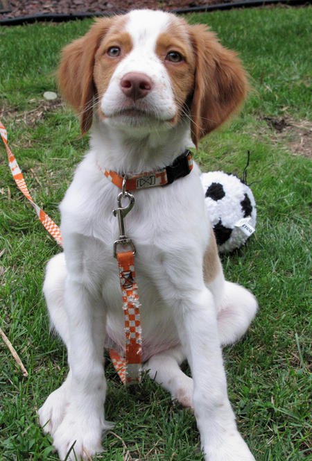
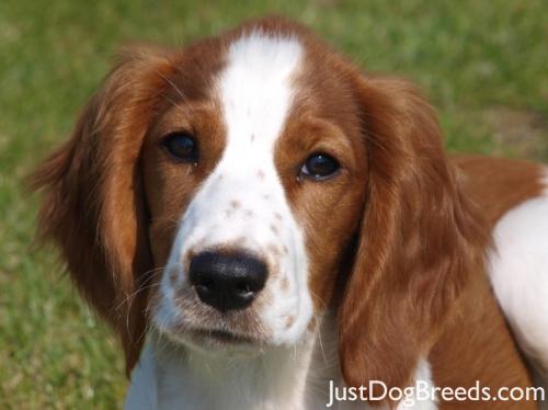
We mention that the task of assigning breed to dogs from images is considered exceptionally challenging. To see why, consider that even a human would have great difficulty in distinguishing between a Brittany and a Welsh Springer Spaniel.
| Brittany | Welsh Springer Spaniel |
|---|---|
 |
 |
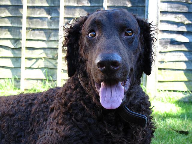
It is not difficult to find other dog breed pairs with minimal inter-class variation (for instance, Curly-Coated Retrievers and American Water Spaniels).
| Curly-Coated Retriever | American Water Spaniel |
|---|---|
 |
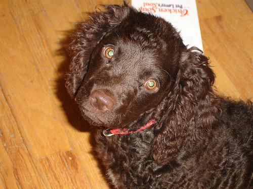 |
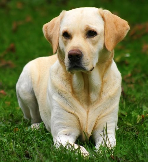
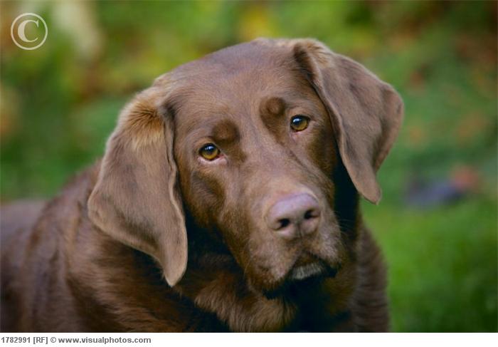
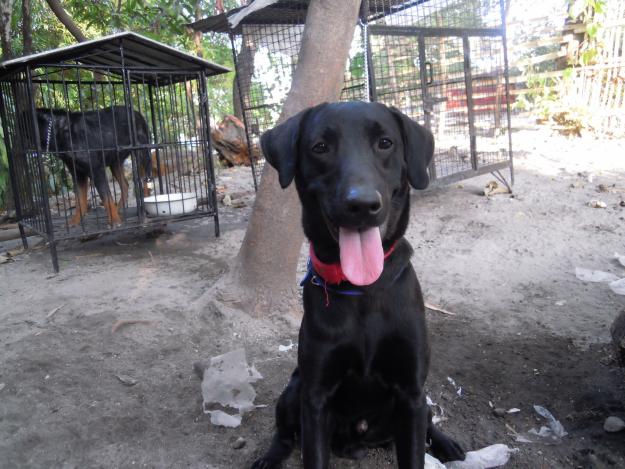
Likewise, recall that labradors come in yellow, chocolate, and black. Your vision-based algorithm will have to conquer this high intra-class variation to determine how to classify all of these different shades as the same breed.
| Yellow Labrador | Chocolate Labrador | Black Labrador |
|---|---|---|
 |
 |
 |
We also mention that random chance presents an exceptionally low bar: setting aside the fact that the classes are slightly imabalanced, a random guess will provide a correct answer roughly 1 in 133 times, which corresponds to an accuracy of less than 1%.
Remember that the practice is far ahead of the theory in deep learning. Experiment with many different architectures, and trust your intuition. And, of course, have fun!
Pre-process the Data
We rescale the images by dividing every pixel in every image by 255.
from PIL import ImageFile
ImageFile.LOAD_TRUNCATED_IMAGES = True
# pre-process the data for Keras
train_tensors = paths_to_tensor(train_files).astype('float32')/255
valid_tensors = paths_to_tensor(valid_files).astype('float32')/255
test_tensors = paths_to_tensor(test_files).astype('float32')/255
(IMPLEMENTATION) Model Architecture
Create a CNN to classify dog breed. At the end of your code cell block, summarize the layers of your model by executing the line:
model.summary()
We have imported some Python modules to get you started, but feel free to import as many modules as you need. If you end up getting stuck, here's a hint that specifies a model that trains relatively fast on CPU and attains >1% test accuracy in 5 epochs:

Question 4: Outline the steps you took to get to your final CNN architecture and your reasoning at each step. If you chose to use the hinted architecture above, describe why you think that CNN architecture should work well for the image classification task.
Answer: I was mostly inspired by the architecture above. I kept the alternation between convolution layers and max pooling layers as advised in the nanodegree lecture. For each convolution layers, I increased the number of filters by a factor of 2 starting at 16 filters for the first convolution layer. I also kept the padding as same because it has been documented that this usually yields better results. A relu activation function was used. For each max pooling layers, the dimensions of the input (height and width) are divided by 2 and those are followed by dropout layers to prevent overfitting. The last layers are a global average pooling followed by a fully connected layer, where the latter contains one node for each dog category (133) and is equipped with a relu activation function.
from keras.layers import Conv2D, MaxPooling2D, GlobalAveragePooling2D
from keras.layers import Dropout, Flatten, Dense
from keras.models import Sequential
model = Sequential()
### TODO: Define your architecture.
model.add(Conv2D(filters=16, kernel_size=2, input_shape=(224, 224, 3), activation='relu', padding='same'))
model.add(MaxPooling2D(pool_size=2, data_format='channels_last'))
model.add(Dropout(0.25))
model.add(Conv2D(filters=32, kernel_size=2, activation='relu', padding='same'))
model.add(MaxPooling2D(pool_size=2, data_format='channels_last'))
model.add(Dropout(0.25))
model.add(Conv2D(filters=64, kernel_size=2, activation='relu', padding='same'))
model.add(MaxPooling2D(pool_size=2, data_format='channels_last'))
model.add(Dropout(0.25))
model.add(GlobalAveragePooling2D())
model.add(Dense(133, activation='relu'))
model.summary()
Compile the Model
model.compile(optimizer='rmsprop', loss='categorical_crossentropy', metrics=['accuracy'])
(IMPLEMENTATION) Train the Model
Train your model in the code cell below. Use model checkpointing to save the model that attains the best validation loss.
You are welcome to augment the training data, but this is not a requirement.
### TODO: specify the number of epochs that you would like to use to train the model.
epochs = 5
### Do NOT modify the code below this line.
checkpointer = ModelCheckpoint(filepath='saved_models/weights.best.from_scratch.hdf5',
verbose=1, save_best_only=True)
model.fit(train_tensors, train_targets,
validation_data=(valid_tensors, valid_targets),
epochs=epochs, batch_size=20, callbacks=[checkpointer], verbose=1)
Load the Model with the Best Validation Loss
model.load_weights('saved_models/weights.best.from_scratch.hdf5')
Test the Model
Try out your model on the test dataset of dog images. Ensure that your test accuracy is greater than 1%.
def test_model(model, test_tensors, test_targets, name):
# get index of predicted dog breed for each image in test set
predictions = [np.argmax(model.predict(np.expand_dims(tensor, axis=0))) for tensor in test_tensors]
# report test accuracy
test_accuracy = 100*np.sum(np.array(predictions)==np.argmax(test_targets, axis=1))/len(predictions)
print('Test accuracy {}: {}%'.format(name, round(test_accuracy, 4)))
test_model(model,test_tensors, test_targets, 'model')
def get_bottleneck_features(path):
bottleneck_features = np.load(path)
train = bottleneck_features['train']
valid = bottleneck_features['valid']
test = bottleneck_features['test']
return train, valid, test
train_VGG16, valid_VGG16, test_VGG16 = get_bottleneck_features('bottleneck_features/DogVGG16Data.bin')
Model Architecture
The model uses the the pre-trained VGG-16 model as a fixed feature extractor, where the last convolutional output of VGG-16 is fed as input to our model. We only add a global average pooling layer and a fully connected layer, where the latter contains one node for each dog category and is equipped with a softmax.
VGG16_model = Sequential()
VGG16_model.add(GlobalAveragePooling2D(input_shape=train_VGG16.shape[1:]))
VGG16_model.add(Dense(133, activation='softmax'))
VGG16_model.summary()
Compile the Model
VGG16_model.compile(loss='categorical_crossentropy', optimizer='rmsprop', metrics=['accuracy'])
Train the Model
checkpointer = ModelCheckpoint(filepath='saved_models/weights.best.VGG16.hdf5',
verbose=1, save_best_only=True)
VGG16_model.fit(train_VGG16, train_targets,
validation_data=(valid_VGG16, valid_targets),
epochs=20, batch_size=20, callbacks=[checkpointer], verbose=1)
Load the Model with the Best Validation Loss
VGG16_model.load_weights('saved_models/weights.best.VGG16.hdf5')
Test the Model
Now, we can use the CNN to test how well it identifies breed within our test dataset of dog images. We print the test accuracy below.
test_model(VGG16_model,test_VGG16, test_targets, 'VGG16')
Predict Dog Breed with the Model
def VGG16_predict_breed(img_path):
# extract bottleneck features
bottleneck_feature = extract_VGG16(path_to_tensor(img_path))
# obtain predicted vector
predicted_vector = VGG16_model.predict(bottleneck_feature)
# return dog breed that is predicted by the model
return dog_names[np.argmax(predicted_vector)]
print(VGG16_predict_breed('images/yuna.jpg'))
print(VGG16_predict_breed('images/tiffany.jpg'))
print(VGG16_predict_breed('images/olivier.jpg'))
Step 5: Create a CNN to Classify Dog Breeds (using Transfer Learning)
You will now use transfer learning to create a CNN that can identify dog breed from images. Your CNN must attain at least 60% accuracy on the test set.
In Step 4, we used transfer learning to create a CNN using VGG-16 bottleneck features. In this section, you must use the bottleneck features from a different pre-trained model. To make things easier for you, we have pre-computed the features for all of the networks that are currently available in Keras:
- VGG-19 bottleneck features
- ResNet-50 bottleneck features
- Inception bottleneck features
- Xception bottleneck features
The files are encoded as such:
Dog{network}Data.npz
where {network}, in the above filename, can be one of VGG19, Resnet50, InceptionV3, or Xception. Pick one of the above architectures, download the corresponding bottleneck features, and store the downloaded file in the bottleneck_features/ folder in the repository.
(IMPLEMENTATION) Obtain Bottleneck Features
In the code block below, extract the bottleneck features corresponding to the train, test, and validation sets by running the following:
bottleneck_features = np.load('bottleneck_features/Dog{network}Data.npz')
train_{network} = bottleneck_features['train']
valid_{network} = bottleneck_features['valid']
test_{network} = bottleneck_features['test']### TODO: Obtain bottleneck features from another pre-trained CNN.
train_VGG19, valid_VGG19, test_VGG19 = get_bottleneck_features('bottleneck_features/DogVGG19Data.bin')
train_Resnet50, valid_Resnet50, test_Resnet50 = get_bottleneck_features('bottleneck_features/DogResnet50Data.bin')
train_InceptionV3, valid_InceptionV3, test_InceptionV3 = get_bottleneck_features('bottleneck_features/DogInceptionV3Data.bin')
train_Xception, valid_Xception, test_Xception = get_bottleneck_features('bottleneck_features/DogXceptionData.bin')
(IMPLEMENTATION) Model Architecture
Create a CNN to classify dog breed. At the end of your code cell block, summarize the layers of your model by executing the line:
<your model's name>.summary()
Question 5: Outline the steps you took to get to your final CNN architecture and your reasoning at each step. Describe why you think the architecture is suitable for the current problem.
Answer:
I selected the Xception model to which I added a global average pooling layer and a fully connected layer with a Softmax activation function and 133 nodes for the 133 dog categories. I trained it for 20 epochs although the best weights were found after only 2 epochs. I chose the Xception model because it allowed me to yield the best test accuracy of 83.8517%. I think this architecture is suitable for the current problem because it has a more efficient use of model parameters than other models and it is known to be already well trained for image classification on ImageNet.
### TODO: Define your architecture.
VGG19_model = Sequential()
VGG19_model.add(GlobalAveragePooling2D(input_shape=(train_VGG19.shape[1:])))
VGG19_model.add(Dense(133, activation='softmax'))
VGG19_model.summary()
Resnet50_model = Sequential()
Resnet50_model.add(GlobalAveragePooling2D(input_shape=(train_Resnet50.shape[1:])))
Resnet50_model.add(Dense(133, activation='softmax'))
Resnet50_model.summary()
InceptionV3_model = Sequential()
InceptionV3_model.add(GlobalAveragePooling2D(input_shape=(train_InceptionV3.shape[1:])))
InceptionV3_model.add(Dense(133, activation='softmax'))
InceptionV3_model.summary()
Xception_model = Sequential()
Xception_model.add(GlobalAveragePooling2D(input_shape=(train_Xception.shape[1:])))
Xception_model.add(Dense(133, activation='softmax'))
Xception_model.summary()
(IMPLEMENTATION) Compile the Model
### TODO: Compile the model.
VGG19_model.compile(loss='categorical_crossentropy', optimizer='rmsprop')
Resnet50_model.compile(loss='categorical_crossentropy', optimizer='rmsprop')
InceptionV3_model.compile(loss='categorical_crossentropy', optimizer='rmsprop')
Xception_model.compile(loss='categorical_crossentropy', optimizer='rmsprop')
(IMPLEMENTATION) Train the Model
Train your model in the code cell below. Use model checkpointing to save the model that attains the best validation loss.
You are welcome to augment the training data, but this is not a requirement.
### TODO: Train the model.
checkpointer = ModelCheckpoint(filepath='saved_models/weights.best.VGG19.hdf5',
verbose=1, save_best_only=True)
VGG19_model.fit(train_VGG19, train_targets,
validation_data=(valid_VGG19, valid_targets),
epochs=20, batch_size=20, callbacks=[checkpointer], verbose=1)
checkpointer = ModelCheckpoint(filepath='saved_models/weights.best.Resnet50.hdf5',
verbose=1, save_best_only=True)
Resnet50_model.fit(train_Resnet50, train_targets,
validation_data=(valid_Resnet50, valid_targets),
epochs=20, batch_size=20, callbacks=[checkpointer], verbose=1)
checkpointer = ModelCheckpoint(filepath='saved_models/weights.best.InceptionV3.hdf5',
verbose=1, save_best_only=True)
InceptionV3_model.fit(train_InceptionV3, train_targets,
validation_data=(valid_InceptionV3, valid_targets),
epochs=20, batch_size=20, callbacks=[checkpointer], verbose=1)
checkpointer = ModelCheckpoint(filepath='saved_models/weights.best.Xception.hdf5',
verbose=1, save_best_only=True)
Xception_model.fit(train_Xception, train_targets,
validation_data=(valid_Xception, valid_targets),
epochs=20, batch_size=20, callbacks=[checkpointer], verbose=1)
(IMPLEMENTATION) Load the Model with the Best Validation Loss
### TODO: Load the model weights with the best validation loss.
VGG19_model.load_weights('saved_models/weights.best.VGG19.hdf5')
Resnet50_model.load_weights('saved_models/weights.best.Resnet50.hdf5')
InceptionV3_model.load_weights('saved_models/weights.best.InceptionV3.hdf5')
Xception_model.load_weights('saved_models/weights.best.Xception.hdf5')
(IMPLEMENTATION) Test the Model
Try out your model on the test dataset of dog images. Ensure that your test accuracy is greater than 60%.
### TODO: Calculate classification accuracy on the test dataset.
test_model(VGG19_model,test_VGG19, test_targets, 'VGG19')
test_model(Resnet50_model,test_Resnet50, test_targets, 'Resnet50')
test_model(InceptionV3_model,test_InceptionV3, test_targets, 'InceptionV3')
test_model(Xception_model,test_Xception, test_targets, 'Xception')
(IMPLEMENTATION) Predict Dog Breed with the Model
Write a function that takes an image path as input and returns the dog breed (Affenpinscher, Afghan_hound, etc) that is predicted by your model.
Similar to the analogous function in Step 5, your function should have three steps:
- Extract the bottleneck features corresponding to the chosen CNN model.
- Supply the bottleneck features as input to the model to return the predicted vector. Note that the argmax of this prediction vector gives the index of the predicted dog breed.
- Use the
dog_namesarray defined in Step 0 of this notebook to return the corresponding breed.
The functions to extract the bottleneck features can be found in extract_bottleneck_features.py, and they have been imported in an earlier code cell. To obtain the bottleneck features corresponding to your chosen CNN architecture, you need to use the function
extract_{network}
where {network}, in the above filename, should be one of VGG19, Resnet50, InceptionV3, or Xception.
### TODO: Write a function that takes a path to an image as input
### and returns the dog breed that is predicted by the model.
def Xception_prediction_breed(img_path):
# extract bottleneck features
bottleneck_feature = extract_Xception(path_to_tensor(img_path))
# obtain predicted vector
predicted_vector = Xception_model.predict(bottleneck_feature)
# return dog breed that is predicted by the model
return dog_names[np.argmax(predicted_vector)]
Step 6: Write your Algorithm
Write an algorithm that accepts a file path to an image and first determines whether the image contains a human, dog, or neither. Then,
- if a dog is detected in the image, return the predicted breed.
- if a human is detected in the image, return the resembling dog breed.
- if neither is detected in the image, provide output that indicates an error.
You are welcome to write your own functions for detecting humans and dogs in images, but feel free to use the face_detector and dog_detector functions developed above. You are required to use your CNN from Step 5 to predict dog breed.
Some sample output for our algorithm is provided below, but feel free to design your own user experience!
(IMPLEMENTATION) Write your Algorithm
### TODO: Write your algorithm.
### Feel free to use as many code cells as needed.
def dog_identification_app(img_path, name):
print ("Hello {}!".format(name))
display(Image(img_path,width=200,height=200))
breed = Xception_prediction_breed(img_path)
if dog_detector(img_path):
print("I believe you are a dog and you look like a {}\n".format(breed))
elif face_detector_opencv(img_path):
print("I believe you are human but you look like a {}\n".format(breed))
else:
print("I can't tell if there's a human or a dog in this picture, can you show me another one ?\n")
Step 7: Test Your Algorithm
In this section, you will take your new algorithm for a spin! What kind of dog does the algorithm think that you look like? If you have a dog, does it predict your dog's breed accurately? If you have a cat, does it mistakenly think that your cat is a dog?
(IMPLEMENTATION) Test Your Algorithm on Sample Images!
Test your algorithm at least six images on your computer. Feel free to use any images you like. Use at least two human and two dog images.
Question 6: Is the output better than you expected :) ? Or worse :( ? Provide at least three possible points of improvement for your algorithm.
Answer: I tested the algorithm on several pictures of dogs. It got the right answer most of the time and it was satisfying. The algorithm is efficient at finding human faces and usually gets it right although it mistook my cat with a human. For the dog breed prediction on a human face, I found the performance variable. It often predicts dachshund although sometimes the ressemblance isn't striking. When I gave it a random objects, it aptly classifies them as neither human nor dog.
Overall the output is better than I expected. One way to improve the algorithm could be to train it on an augmented dataset. Also it would be nice to have a more accurate model for human faces predictions (it often thinks that cats are humans). Finally, it would be nice to have a wider variety of dog breeds. On the application side it would be nice to return a picture of a corresponding dog that looks like the human on the input picture.
## TODO: Execute your algorithm from Step 6 on
## at least 6 images on your computer.
## Feel free to use as many code cells as needed.
dog_identification_app('images/pomeranian.jpg', 'Pomeranian')
dog_identification_app('images/yuna.jpg', 'Yuna')
dog_identification_app('images/olivier.jpg', 'Olivier')
dog_identification_app('images/tiffany.jpg', 'Tiffany')
dog_identification_app('images/katoun.jpg', 'Katoun')
dog_identification_app('images/toaster.jpg', 'Toaster')


